Mathematical modeling is an integral part of understanding the feasibility of our project. Here, for MOLDEMORT, we have attempted to model extremely crucial components of our project using mathematical equations to predict how our chimeric protein may work in-vitro. We have provided all the equations that have been in use, along with our understanding of the requirements of the models. The data thus obtained can be further used to design experiments in the wet lab.
The team has identified seven fungal species through morphology and Sanger sequencing. To check the activity of our chitinase enzymes, we need to determine the growth rate and lag phase of the species to compare it with the changed parameters when inflicted with the extracted protein.
To analyze the growth of the fungus, two different methods were used:
When grown on a Petri plate in a PDA (Potato dextrose agar) medium, fungus tends to grow radially (given no contamination). The increasing radius and hence the increasing surface area is a parameter that can be used to check its growth rate over time.[1]
The unidentified samples were inoculated on Petri plates and observed for 4-5 days to capture images of the growing fungus. It was assumed that inoculum for all fungal species was of equal size. The images were aligned and analyzed using the ImageJ software, where the radius and the corresponding area were measured.
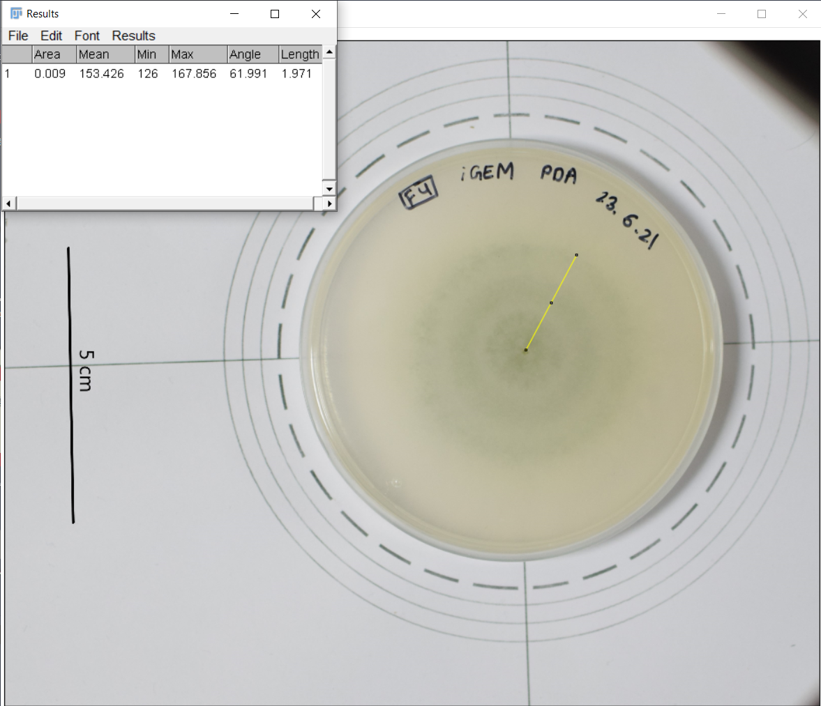
Figure 1. Unannotated image, not resized yet
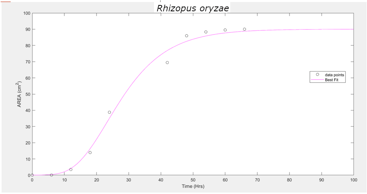
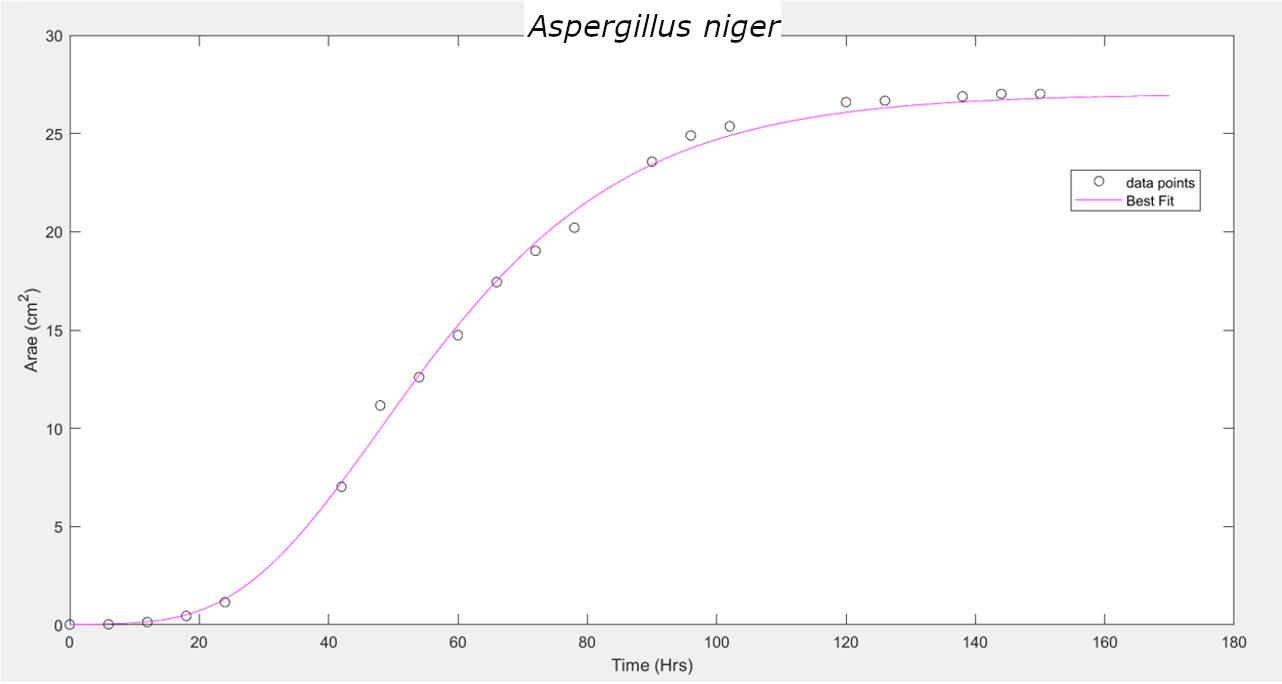
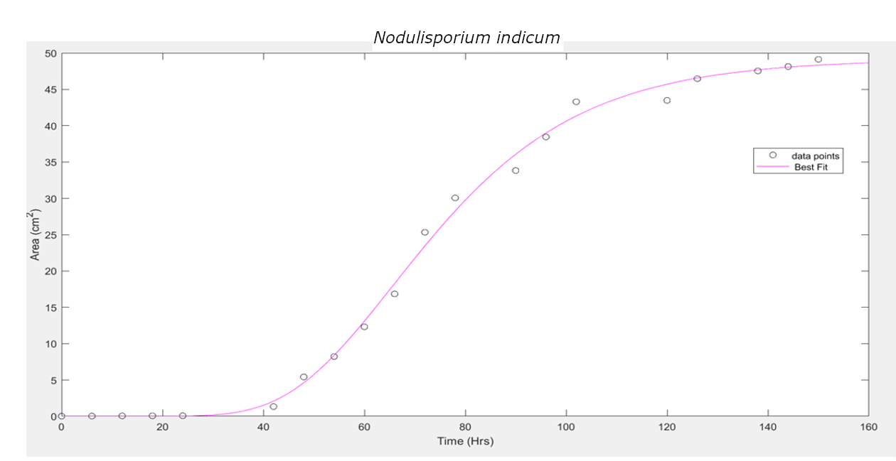
The team has considered several growth models, which were mostly used for bacterial growth, yet can be used for fungal growth as well.[2][3]
These three equations were used to fit the curve and find the unknown parameters. It has been observed that the Gompertz model of growth gives us the least RMSE (Root Mean Squared Error), hence proving to be the best model for our data.
| Fungus Sample | Goodness of fit | SSE | R-square | Adjusted R-square | RMSE | \(\mu\) (max growth rate) in \(cm^2/hr\) | \(\lambda\) (lag time) in \(hr\) | \(\beta\) |
|---|---|---|---|---|---|---|---|---|
R. oryzae |
Gompertz |
98.28 |
0.9934 |
0.9925 |
3.505 |
3.319 |
23.42 |
0.2167 |
Richards |
109.8 |
0.9926 |
0.9917 |
3.693 |
1.402 |
13.32 |
||
Logistic |
180.2 |
0.9879 |
0.9863 |
4.746 |
3.303 |
14.04 |
||
A. niger |
Gompertz |
3.982 |
0.9982 |
0.9981 |
0.4704 |
0.4765 |
47.95 |
0.048 |
Richards |
3.951 |
0.9982 |
0.998 |
0.4821 |
0.05567 |
26.28 |
||
Logistic |
12.64 |
0.9942 |
0.9939 |
0.8378 |
0.4471 |
27.46 |
||
N. indicum |
Gompertz |
25.43 |
0.9966 |
0.9964 |
1.188 |
0.8935 |
65.78 |
0.2167 |
Richards |
28.72 |
0.9962 |
0.996 |
1.263 |
0.3809 |
45.27 |
||
Logistic |
60.19 |
0.992 |
0.9915 |
1.829 |
0.8587 |
46.42 |
SSE: Sum of squared estimate of errors ; RMSE: Root Mean Squared Error
The surface area based growth model was conducted before the completion of fungal identification. The names have been assigned after its identification.
Unannotated image, not resized yet
Unannotated image, not resized yet
Unannotated image, not resized yet
Few drawbacks in this method:
Scattering of light by a replicating population over time, and hence the changing OD is a good proxy for the growth of fungus instead of measuring its changing radius.[4]
The fungal species were grown in a 96-well plate in a PDB (Potato dextrose broth) medium, with spores suspended in 1X PBS (Phosphate buffered saline), and observations were taken 4-5 days for an interval of 6 hours at 605nm. The assumption is made that the spore suspension has been uniformly distributed throughout the well.
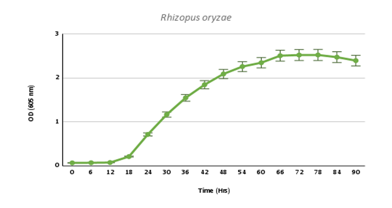
Figure 1. Unannotated image, not resized yet
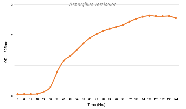
Figure 1. Unannotated image, not resized yet
| Growth rate (Absorbance/hr) | Lag time (hr) | |
|---|---|---|
Rhizopus oryzae |
0.3145 |
27.69 |
Aspergillus versicolor |
0.1701 |
42.72 |
Limitations of this method:
These growth models would be needed to compare the changing growth rate and lag time when the fungal species is administered with our designed chitinases. A slower growth rate and higher lag time would help us to support our alternate hypothesis of developing chimeric chitinases with enhanced antifungal activity than wild-type chitinases.
Nipagin, being a methylparaben, is an antifungal agent primarily used in cosmetics and food preservatives.[5]
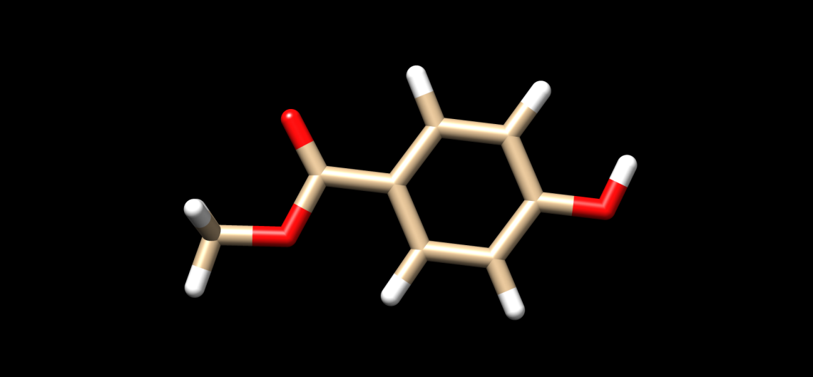
Figure 1. Unannotated image, not resized yet
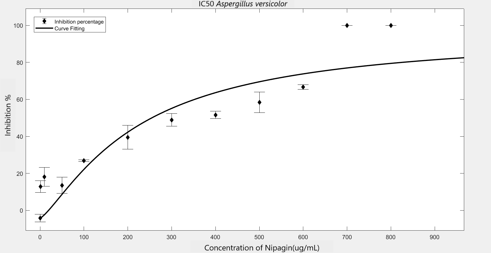
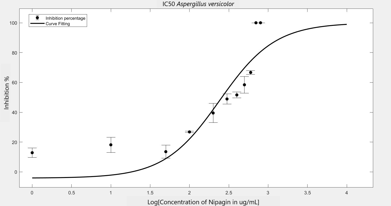
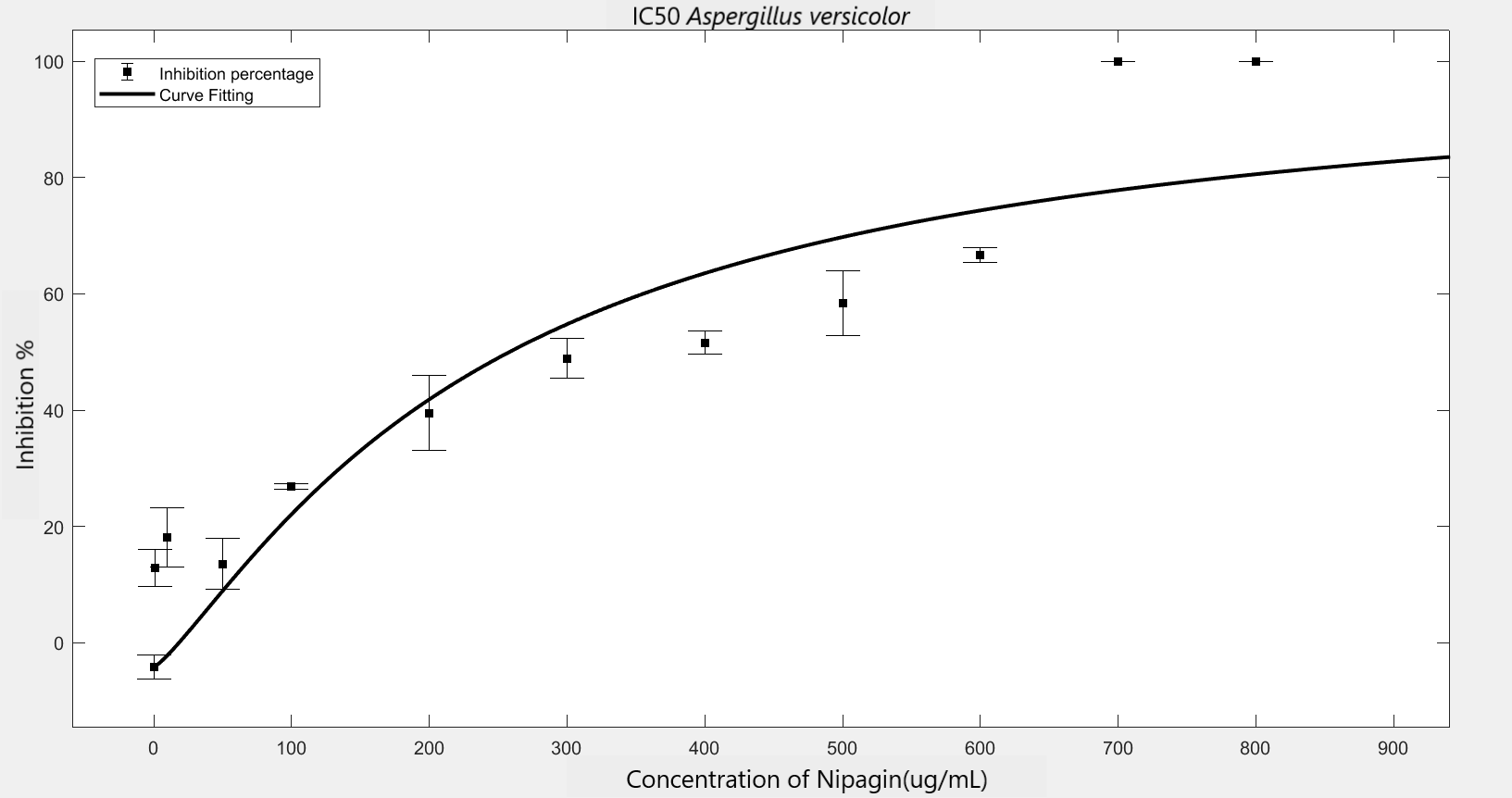
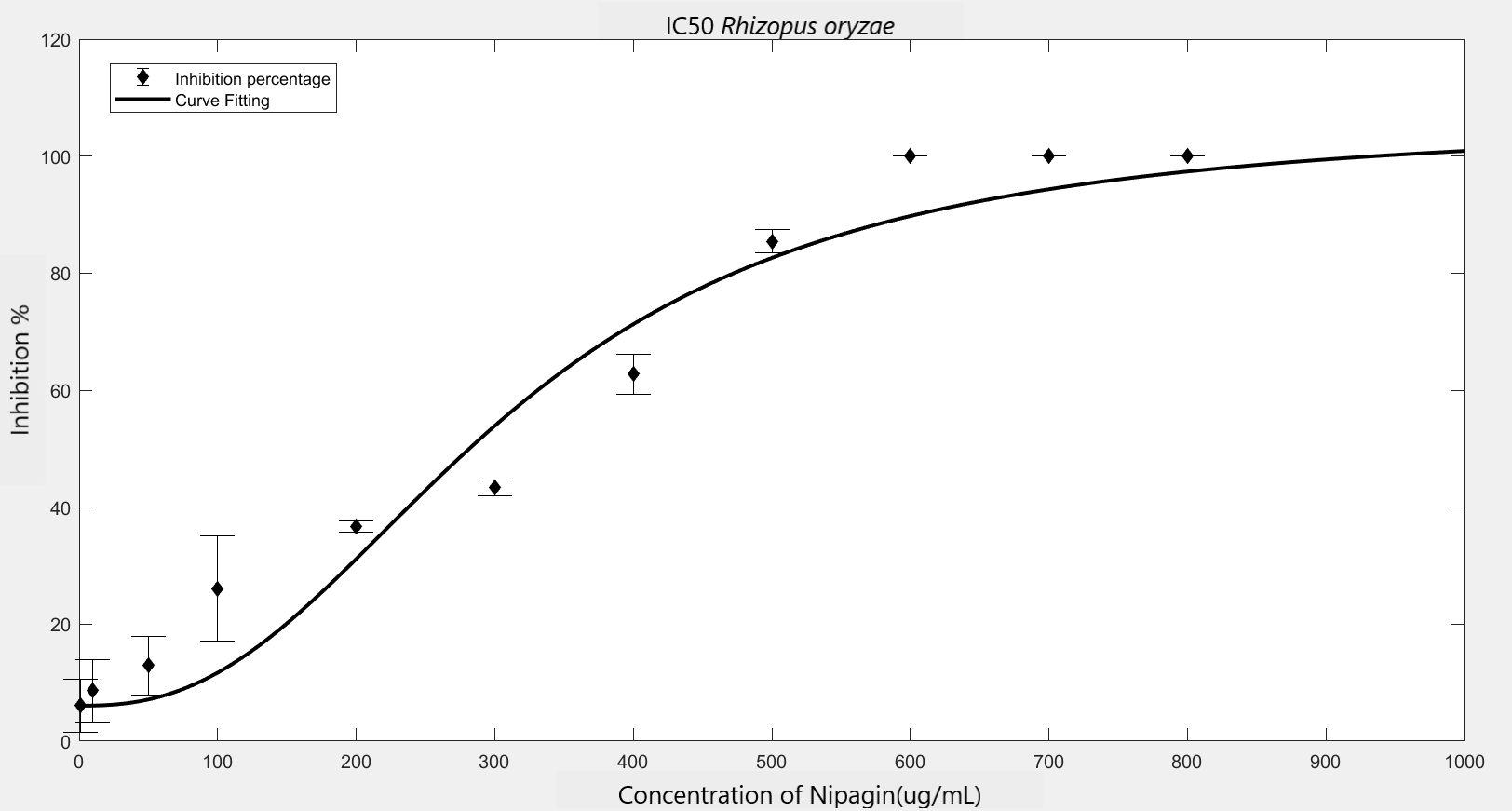
We carried out an antifungal assay using Nipagin to calculate its IC50 for the fungal species identified by the team. This same experiment would be repeated with the purified protein of our interest to calculate its IC50 for different fungal species. We wish to check the applicability of the models which calculate IC50 using Nipagin, which then would be used for our protein.
IC50 of the antifungal here would indicate how much of the chemical would be needed to inhibit the in vitro growth of the given fungal species by 50% [6]. Lower the IC50, better the efficiency of the antifungal.
An initial trial in experimenting, with antifungal concentration starting from 1000μg/mL, with serial dilutions of ½ till the final concentration of 0.488μg/mL gave us the IC50 as follows: Rhizopus oryzae (230.46μg/mL) and Aspergillus versicolor (288.916μg/mL)
The experiment was repeated to verify the results with different mathematical methods. Since the IC50 of Nipagin for both the fungus came in about 200-300μg/mL range, the graduation of nipagin concentration was changed to 800μg/mL to 0.5μg/mL, diluting it by 100μg/mL for the initial concentrations.
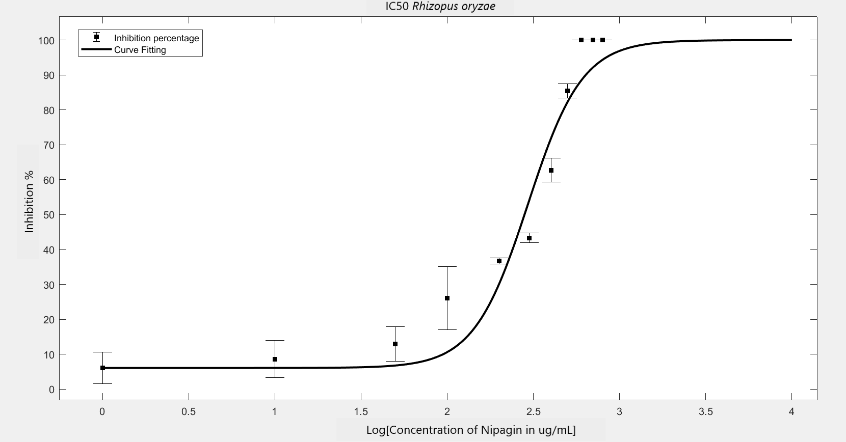
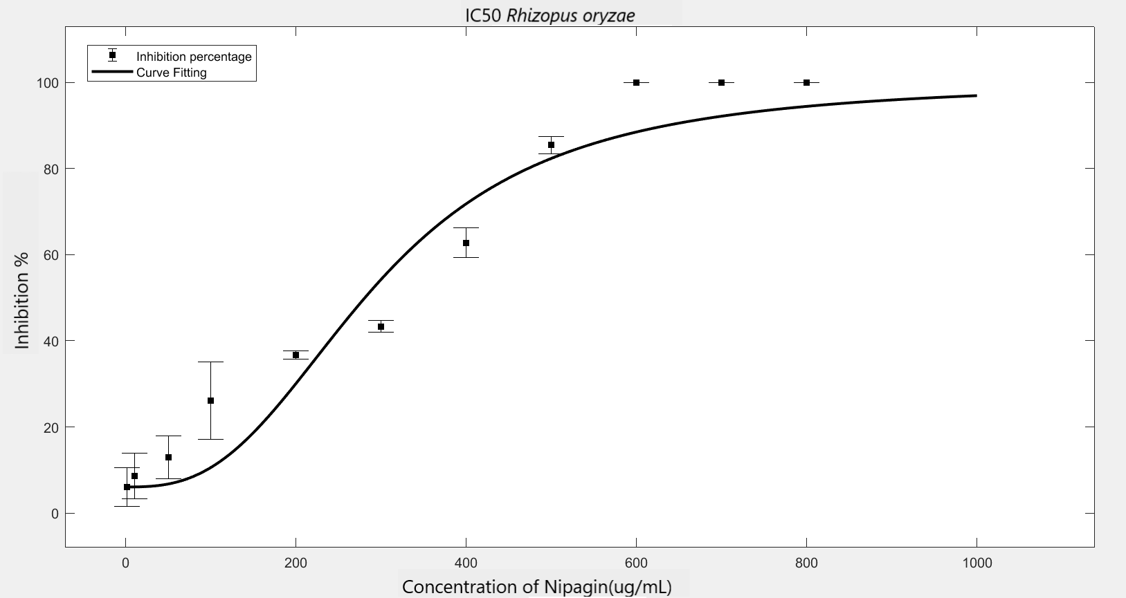
The inhibition percentage has been calculated using three different methods:[7]
Where,
\[I_{min}=\text{Lowest Inhibition}\] \[I_{max}=\text{Highest Inhibition}\]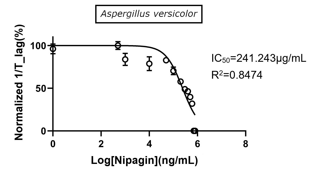
Figure 1. Unannotated image, not resized yet
Unannotated image, not resized yet
Unannotated image, not resized yet
Unannotated image, not resized yet
| Method Used | Hill coefficient | \(IC_{50}\) (\(μg/mL\)) |
|---|---|---|
Method 1 |
1.2785 |
223.534 |
Method 2 |
1.2308 |
241.9844 |
Method 3 |
1.2308 |
241.9797 |
Using GraphPad |
-1.23 |
241.243 |
(R2=0.8474) |
||
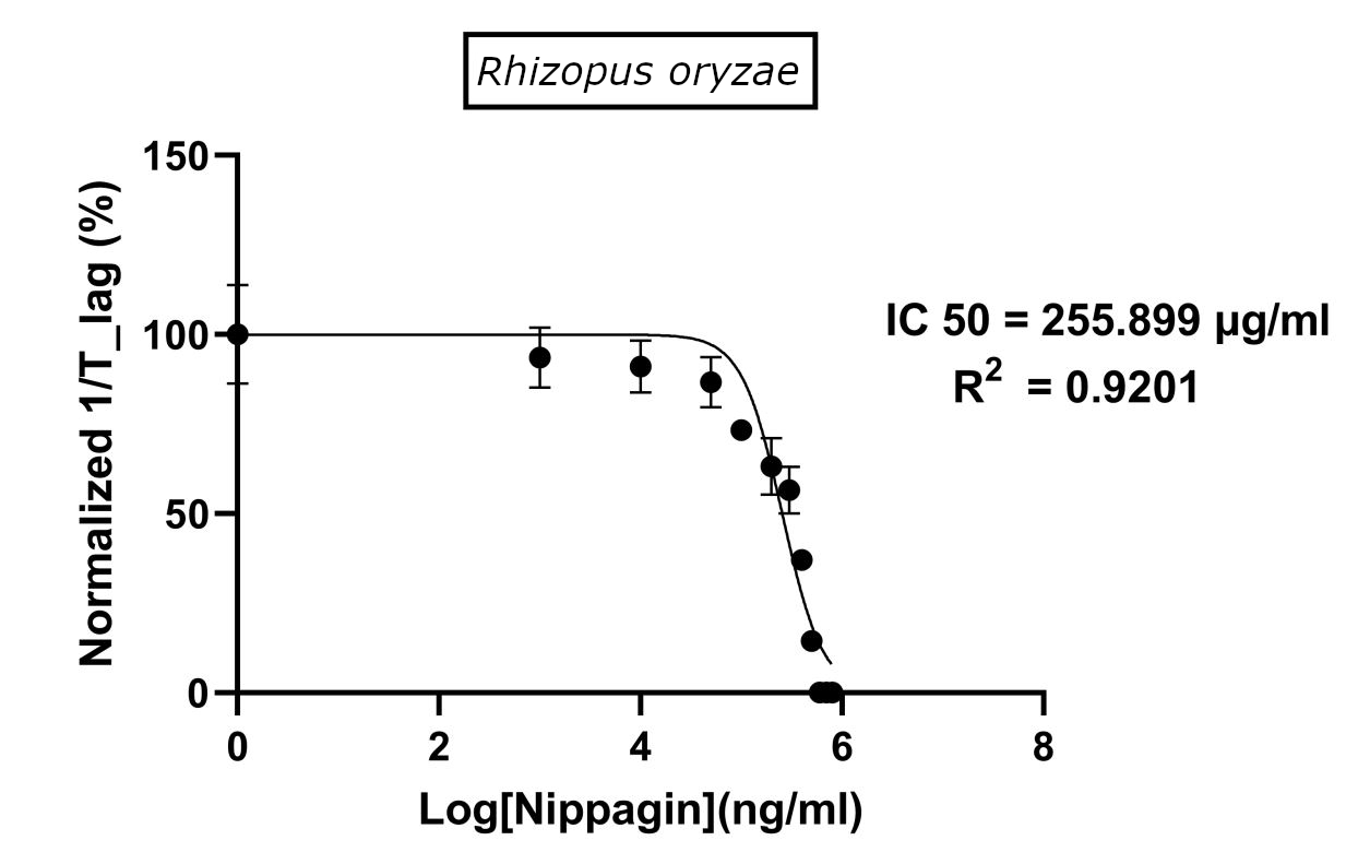
Figure 1. Unannotated image, not resized yet
Unannotated image, not resized yet
Unannotated image, not resized yet
Unannotated image, not resized yet
| Method Used | Hill coefficient | \(IC_{50}\) (\(μg/mL\)) |
|---|---|---|
Method 1 |
2.4848 |
231.6738 |
Method 2 |
2.7604 |
294.2999 |
Method 3 |
2.7604 |
294.2999 |
Using GraphPad |
-2.172 |
255.899 |
(\(R^2\) = 0.9202) |
||
Chitinase-chitin interaction can be considered as a ligand-receptor interaction, where the chitin polymer acts as a ligand that binds to the active sites of the chitinase protein, acting as receptors. The docking of the chitin octamer to the chimeric chitinases had already been demonstrated through Autodoc results, which provides us with the binding energy. The binding energy can be used to calculate the dissociation constants,Kd using the equation:
\[\begin{equation} \Delta G=RT \cdot lnK_{d} \end{equation}\]Here, the ligand is the chitin polymer, of which the cell wall of fungi is made of. The receptor is the active site of the chitinase protein. Formation of ligand-receptor complex is given by:
\[L+R \underset{k_2}{\stackrel{k_1}{\rightleftharpoons}} L-R\]This complex is formed by the virtue of non-covalent bonds like hydrogen bonding, electrostatic bonding, etc. The forward rate is given by \(k_1[L][R]\) and reverse rate is given by, \(k_2[L-R]\). Rate of change in the concentration of the ligand-receptor complex is given by,
\[\begin{equation} \frac{d[L-R]}{dt}=k_1[L][R]-k_2[L-R] \tag{1} \end{equation}\]Considering 1:1 ratio of ligand and receptor entity, we have,
\[\begin{equation} \frac{d[L]}{dt}=\frac{d[R]}{dt}=-k_1[L][R]+k_2[L-R] \end{equation}\]At the steady state,
\[\begin{equation} \begin{aligned} &\frac{d[L-R]}{dt}=0\\ \implies & k_1[L][R]-k_2[L-R]=0\\ \implies &\frac{k_1}{k_2}=\frac{[L-R]}{[L][R]}=k_{eq} \end{aligned} \end{equation}\]The affinity of the ligand is usually represented by the dissociation constant, \(K_d=\frac{1}{k_{eq}}\)
Considering the total concentration of ligand and total concentration of receptor to be constant for a small period of time, we have
\[\begin{equation} [L]=[L]_T-[L-R] \tag{2} \end{equation}\] \[\begin{equation} [R]=[R]_T-[L-R] \tag{3} \end{equation}\]Substituting [2] and [3] in equation [1], we have,
\[\begin{equation} \frac{d[L-R]}{dt}=k_{1}\left([L]_{T}-[L-R]\right)\left([R]_{T}-[L-R]\right)-k_{2}[L-R] \end{equation}\] Where,| Chitinase type | Ligand-Receptor complex concentration |
|---|---|
Plant chitinase combo 1 |
0.957205 |
Plant chitinase combo 2 |
0.94672139 |
Barley |
0.93794263 |
Wheat |
0.83258658 |
Bacterial chitinase combo 1 |
0.92756562 |
Bacterial chitinase combo 2 |
0.93296366 |
Serratia marcescens |
0.96870234 |
Streptomyces orientalis |
0.8934335 |
The graph has been plotted using JSim Version 2 software, by putting all the required values. The code can be found here.
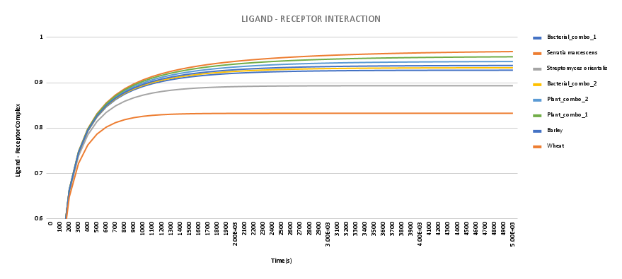
Figure 1. Binding activity of the recombinant
From the graph and the concentration of the Ligand-Receptor complex, it can be concluded that adding binding domains from a high-efficiency chitinase to Catalytic domains of low-efficiency chitinase increases the binding efficiency of low-efficiency chitinase, and thus the recombinant chitinase has higher binding efficiency than its parent wild type chitinase.
Note: This model depicts the binding activity of the protein to chitin octamer; itThe backward does not show the antifungal activity of the engineered protein, as only chitin polymer is taken into consideration, rather than the complex cell wall of the fungus.
We tried to estimate the amount of IPTG that would be required for the optimal protein production so as to predict and thereby help with the experimental design.
We also predicted the max amount of protein that a single E.coli cell would be able to produce and further went on to verify our predictions with experimental results. To get IPTG vs Protein output and Time vs Max Protein output curve, we tried modeling every metabolic process that takes place inside the cell after IPTG induction that is responsible for the production of our enzyme.
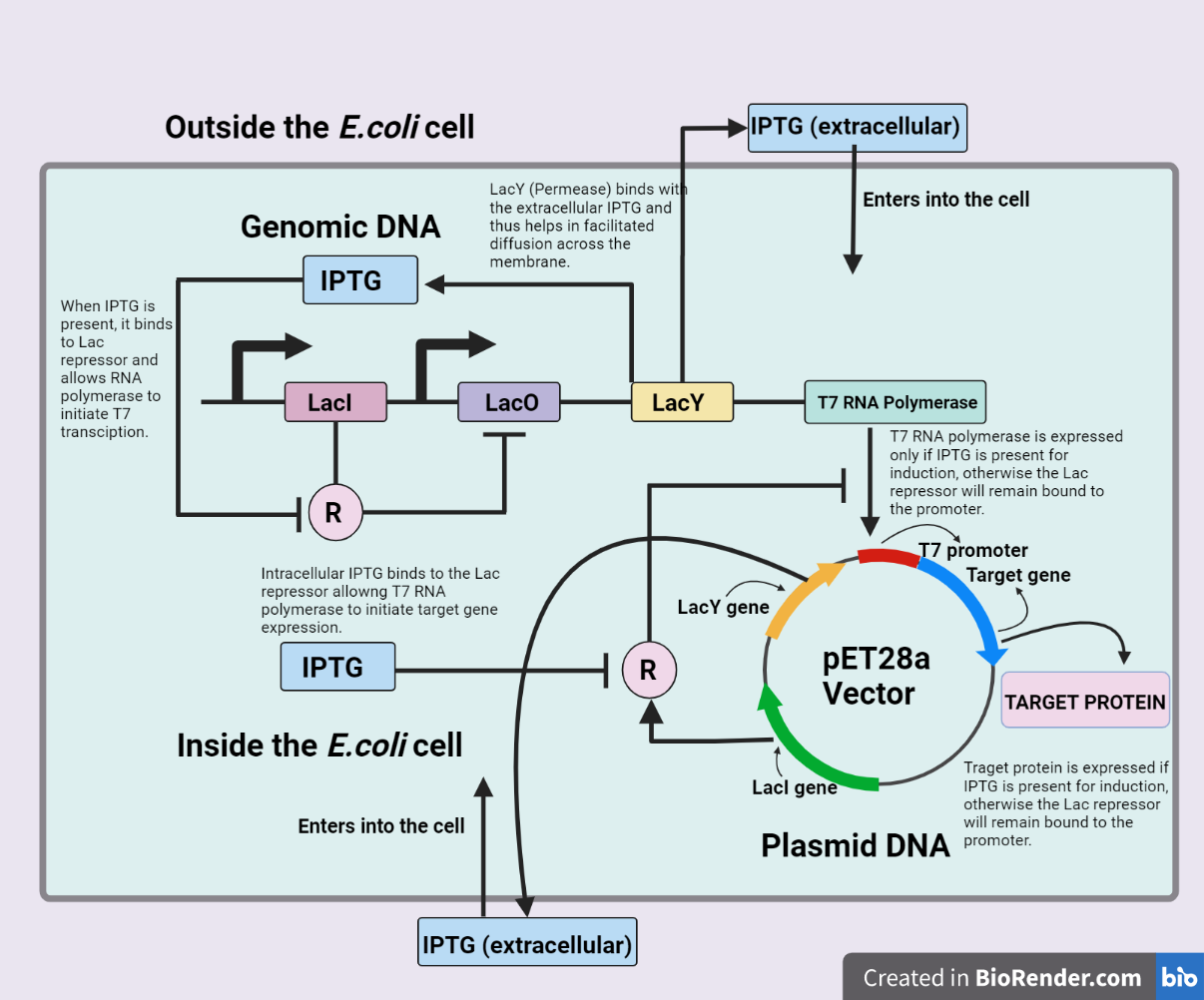
Figure 1. Unannotated image, not resized yet
The gene of our interest is expressed in the BL21 DE(3) strain of E.coli bacteria, whose expression will be under the inducible promoter. The inducer here is IPTG (Isopropyl β-d-1-thiogalactopyranoside). The T7 RNA polymerase which binds to the promoter of our gene of interest and helps in transcription is further under the control of the Lac operon. The IPTG thus have to bind with both:
The metabolic processes for Enzyme production are described in terms of the following Ordinary differential equations (ODEs):[9]
| Symbol | Description |
|---|---|
[\(mRNA_{LacI}\)] |
mRNA of LacI |
[LacI] |
LacI |
[\(IPTG_{in}\)] |
Intracellular IPTG |
[\(IPTG_{ex}\)] |
Extracellular IPTG |
[\(mRNA_{LacY}\)] |
mRNA of LacY |
[LacY] |
LacY |
[\(LacY - IPTG_{ex}\)] |
\(LacY - IPTG_{extracellular}\) complex |
[\(LacI - IPTG_{in}\)] |
\(LacI - IPTG_{intracellular}\) complex |
[\(LacI_{F}\)] |
Free (unbounded) LacI |
[\(mRNA_{\text{T7 RNA POL}}\)] |
mRNA of T7 RNA polymerase |
[T7 RNA POL] |
T7 RNA polymerase |
[T7 \(RP_{B}\)] |
T7 RNA polymerase bound to promoter region |
[\(mRNA_{\text{chitinase}}\)] |
mRNA of Chitinase |
[Chitinase] |
Chitinase |
Note: The elements for the plasmid part are represented with the same Symbols but have an additional “P” added to them to signify plasmid.
| Symbol | Description | Value |
|---|---|---|
K_{tcI} |
Rate constant for transcription of LacI |
0.23nMmin^(-1)[9] |
K_{PtcI} |
||
K_{dmI} |
Degradation constant of LacI mRNA |
0.462 min^(-1)[9] |
K_{PdmI} |
||
K_{tl} |
Rate constant for translation of LacI |
15 min^(-1)[9] |
K_{Ptl} |
||
K_{dpI} |
Degradation constant for LacI |
0.2 min^(-1)[9] |
K_{PdpI} |
||
K_{pdiff} |
Rate constant for passive diffusion of IPTG |
0.92 min^(-1)[9] |
K_{Ppdiff} |
||
K_{fdiff} |
Rate constant of facilitated diffusion |
6*10^4 min^(-1)[9] |
K_{Pfdiff} |
||
K_{fY} |
Forward reaction rate constant for formation of LacY - IPTG complex |
0.12nM^(-1)min^(-1)[9] |
K_{PfY} |
||
K_{bY} |
Backward reaction rate constant for the formation of LacY - IPTG complex |
0.1 min^(-1)[9] |
K_{PbY} |
||
K_{dYI} |
Degradation constant for LacY - IPTG complex |
0.2 min^(-1)[9] |
K_{PdYI} |
||
K_{fI} |
Forward reaction rate constant for formation of LacY - IPTG(intracellular) complex |
0.12 nM^(-1)min^(-1)[9] |
K_{PfI} |
||
K_{bI} |
Backward reaction rate constant for formation of LacI - IPTG(intracellular) complex |
12 min^(-1)[9] |
K_{PbI} |
||
K_{tcY} |
Rate constant for transcription of LacY |
0.5nMmin^(-1)[9] |
K_{PtcY} |
||
K_{dmY} |
Degradation constant of LacY mRNA |
0.462 min^(-1)[9] |
K_{PdmY} |
||
K_{tlY} |
Rate constant of translation of LacY |
30 min^(-1)[9] |
K_{PtlY} |
||
K_{dY} |
Degradation constant for LacY |
0.2 min^(-1)[9] |
K_{PdY} |
||
K_{tcT7} |
Rate constant of transcription of T7 RNA Pol |
0.5 nMmin^(-1)[9] |
K_{dmT7} |
Degradation constant of T7 RNA Pol mRNA |
0.462 min^(-1)[9] |
K_{aff} |
Affinity constant of LacI to the operator region |
0.2 min^(-1)[9] |
K_{tlT7} |
Rate constant of translation of T7 RNA Pol |
6.116 min^(-1)[9] |
K_{dpT7} |
Degradation constant of T7 RNA Pol |
0.462 min^(-1)[9] |
K_{b} |
Binding constant of T7 RNA to Promoter |
0.22 min^(-1)[9] |
K_{ub} |
Unbinding constant |
28.8 min^(-1)[9] |
K_{leaky} |
Rate constant for leaky expression |
0.01 nMmin^(-1)[9] |
K_m |
Michaelis Menten constant |
3*10^5 nM[9] |
K_1 |
Transcription Rate constant of Chitinase mRNA |
2.3658 * 10^3 nMmin^(-1)[9] |
K_{dm_chitinase} |
Degradation Rate constant for Chitinase mRNA |
0.462min^-1[9] |
K_{tl_chitinase} |
Translation Rate constant for Chitinase |
10 min^-1[9] |
K_{dp_chitinase} |
Degradation constant for chitinase |
0.2 min^-1[9] |

Figure 1. Unannotated image, not resized yet
Through our model, we were able to predict that at the concentration of 0.1 - 1 mM IPTG, we can obtain optimal protein production. This prediction helped us in the design of experiments concerning the expression of the protein. It must be noted that these predictions are well in line with the standard procedures that are being used for IPTG induction.
Our other area of interest was predicting the total amount of enzyme that could be produced by a single E Coli: Through experimental data, we got to know that 2 litres of culture produce about 20 mg of protein. Assuming there are 10^10 bacteria / L [10] of culture (general assumption) we were able to calculate the amount of protein produced by a single E.coli to be ~ 256000 nM. These experimental results are very close to our prediction which is 255853.577 nM/ cell.

Figure 1. Unannotated image, not resized yet
Since our chimeric Chitinase comprises domains from two different chitinases, with both of them having a binding domain, we could, in theory, predict the activity of our chitinase by analyzing the binding of the substrate with individual domains and further coupling the activity to get a combined activity.[11]
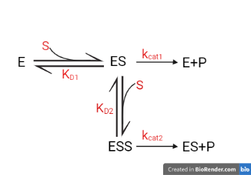
Figure 1. Unannotated image, not resized yet
We here analyse the activity of bacterial Chitinase combo 2 consisting of domains from two chitinases - Serratia marcescens chitinase and Streptomyces orientalis chitinase. Here instead of Streptomyces orientalis we have used proxy species of the same genus Streptomyces griseus as the literature data for Streptomyces orientalis was unavailable. The dissociation constants and Vmax for both chitinases were determined from the literature survey.[12][13]
K_{D1} |
3.36*10^(-5) |
K_{D2} |
4.43*10^(-6) |
Vmax1 |
0.18mmol/min |
Vmax2 |
2.4mmol/min |
The Vmax for chitinase was found to be 2.3739 mmol/min, which gives us an idea of how adding domains from high activity enzymes could in theory improve the efficiency of low activity enzymes.
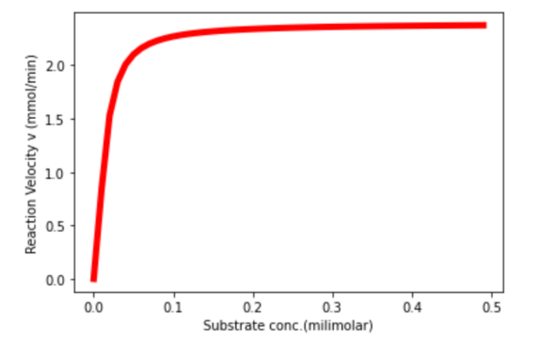
Figure 1. Unannotated image, not resized yet
Further plotting Lineweaver Burk Plot:

Figure 1. Unannotated image, not resized yet
For the delivery of our chimeric chitinase into the human system, we are looking forward to proposing/ using nanoparticles (specifically PLGA) that are suitable due to their ability for controlled drug release, improved therapeutic efficiency, and reduction in the dose of drug administered.
Upon doing assays using our engineered chimeric protein, we have found that our protein is stable at room temperature and shows promising activity.Thus, it further strengthens our proposal to use PLGA as a delivery molecule to the human body.
PLGA - Poly(lactic-co-glycolic acid) is a synthetic copolymer made up of Lactic Acid (LA) and glycolic Acid(GA) and is extensively used for controlled drug delivery(approved by FDA). In an aqueous environment, the chain undergoes a hydrolytic attack on its ester bonds and degrades into LA and GA which are endogenous compounds normally metabolized through the Krebs cycle. By changing the LA/GA ratio and molecular weight in the polymer we could easily control the degradation time of the molecule. The degradation of the PLGA microsphere typically starts at the center of the sphere and the degradation front moves outwards.
Here we are trying to model and predict the degradation kinetics of PLGA (LA/GA ratio 50:50 and Mw 41.9 KDa in human body which helps us understanding the controlled drug release in human body.
Protein release from PLGA Microsphere(MS) is an autocatalytic polymer degradation mechanism, involving 3 prominent steps:[14]
Assumptions made
PLGA degradation governs protein solubilization and release. PLGA degradation is promoted in the MS center due to the polymer autocatalytic degradation mechanism, causing a decrease in pH and enhancing the degradation process.
\[\begin{equation} \rho=\frac{r}{R_{MS}} \tag{1} \end{equation}\] Where,Note: \(B_0,t_{ind}, \psi\) are all adjustable parameters.
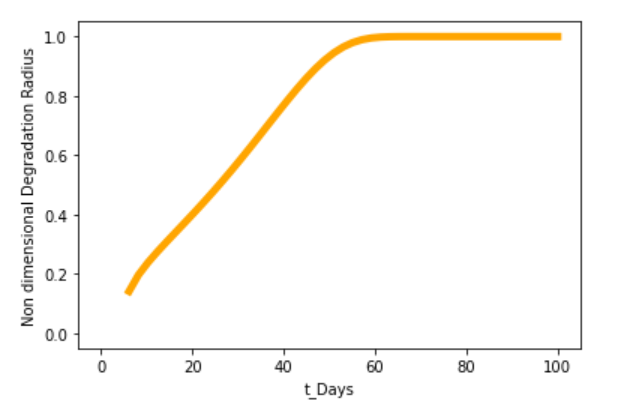
Figure 1. Unannotated image, not resized yet
This model predicts that our PLGA microsphere(Mw = 41.9 KDa) will undergo full disintegration in about 60 days (2 months) in physiological conditions. The rate of protein release will be in proportion with the decay rate of the microsphere and hence the dynamics of protein released could be analyzed using this model.